The experimental set-up and results covered in this post can be found here: 10.5281/zenodo.1233602.
Lately, I’ve been helping Rachel Harding, a fellow postdoc at SGC and one of the pioneers of the Extreme Open Science Initiative at SGC, with some HTT experiments. She is also working on HTT, and has in fact been working on HTT way longer than I have. Read more about her work here: http://labscribbles.com/.
Rachel has been working on a publication on a toolkit to enable people to more easily purify and study HTT and she has very kindly included me to help show the expression of the HTT constructs by Western blot. You can read a draft of the manuscript here: https://zenodo.org/record/1194724#.Ws9pli7wapp.
The work here is slightly different from what I have been doing previously. I usually express these constructs in mammalian cells and harvest whole cell lysates, after which I quantify the total amount of protein using a bicinchoninic acid assay (BCA assay). I then normalise the protein concentrations of all my samples and carry out my Western blot, probing for my protein of interest (eg, HTT) and a housekeeping protein such as GAPDH, which should be equally abundant across all samples after normalisation and ensures that any differences in abundance of my protein of interest are due to the treatment and not due to improper loading.
For this experiment, Rachel provided me with purified HTT protein. As such, we cannot use the BCA assay or a housekeeping protein to normalise the samples, so we’ll need to manually adjust the volumes of protein loaded after each Western blot. For the first run, as I did not know what to expect, I ran equal volumes of each construct just to see how the relative concentrations were like across the samples.
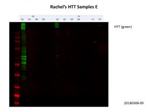
As you can see, the protein concentrations were very variable across the samples. As with my previous experiments, the constructs D1 to D6 are as follows:
D1: 23 Q repeats
D2: 54 Q repeats
D4: 79 Q repeats
D6: 145 Q repeats
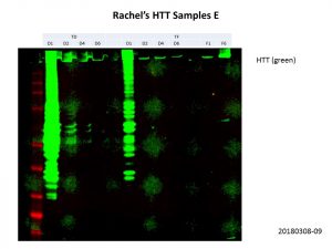
In agreement with my previous experiment in mammalian cells, the D1 construct could be detected for both the transduction (TD) and transfection (TF) samples, but the other samples were much more diluted compared the D1 samples. Here’s an overexposed image, we can see some protein in the other lanes but the background is too high to quantify the band intensities accurately.
Luckily, Rachel provided me with some concentrated samples as well, so I used these for the D2, D4 and D6 constructs AND diluted down the unconcentrated D1 constructs. Here’s my second go at it.
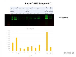
Better but not quite there yet, so I did some quantification of the bands and normalisation of the loading volumes. After several more runs of quantification and normalisation, this was my final run!
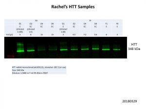
Unfortunately, this was the best I could get. The D4 and D6 transduction samples were still fainter compared to the other samples, but clear bands can be seen in all samples. I could reduce the amount of protein I load for the other samples to levels similar to that of the D4 and D6 samples but all the bands would be fainter. We’ll see what Rachel makes of this and decide how to proceed.